Wrapping up Learning Chess Biases and Proposed Next Steps

Introduction

Today is the final day of my first rotation with CJ and as part of the rotation requirements, I need to write a final report. In line with some of my other assignments, I've decided to complete this in the form of a blog! This post will contain three parts: a brief literature review, a summary of the work from the rotation, and potential next steps for this research. If you've been following my blog for the last month, you would probably have already seen most of this content, but I'll put it here again for the sake of completeness.

Literature Review

Reinforcement Learning (RL) is an area of research in computer science which gained a significant amount of starting in the 1980’s and 1990’s (Kaebling et al.). RL aims to learn an optimal strategy for agent to solve a task using known rewards and punishments for the given domain, without needing to specify how the tasks must be solved. Inverse Reinforcement Learning (IRL) introduced by Ng and Russell in 1998 aims for the opposite phenomenon – watching an agent perform an optimal strategy and learning the (unknown) rewards that the agent is using to solve the task. Ng and Russel give two primary motivations for IRL – learning how humans (or animals) operate in a complicated domain and constructing an agent which can behave successfully in a given domain.

However, traditional IRL requires a key assumption that the agent is performing its task optimally, and this is not a valid assumption that we can make when observing humans, as humans are intrinsically biased, and systematically deviate from optimality. A number of recent papers have been published exploring the idea of learning the rewards of biased agents. For example, Evans et al. published a paper learning the rewards of a biased agent suffering from hyperbolic discounting, Majumdar and Pavone published a paper studying biased agents which were overconfident or underconfident about probabilistic outcomes, and Reddy et al. published a paper learning the rewards of biased agents which held incorrect assumptions about the environment state.

While these papers’ preliminary results showed promise in learning the reward functions of biased agents, each of these models held specific assumptions on the nature of the bias, which could lead to even worse results than traditional IRL if the model’s assumption about the nature of the bias was incorrect.

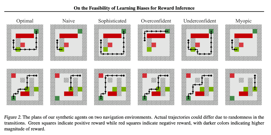
In 2019, Shah et al. explored a new approach, to see if these biases could be learned during the model along with the reward function. Using several novel techniques for this application, such as the use of a value iteration network and pretraining near-optimal agents from a subset of known rewards, the authors were able to achieve a slight improvement in agent understanding for a toy gridworld domain. In addition, the authors claim that with an improvement in available differentiable planners, this method would work even better.

Completed Work

The prior literature in biased IRL has mainly focused on artificially constructed “toy” domains, due to their simplicity in both state-space and ease of generating new data. However, because the entire motivation of studying biased IRL comes from its potential applications in observing human data, we decided to apply biased IRL to an actual human domain. After brainstorming several possible domains, we decided to work on chess. Chess has several benefits as domain for this purpose:

• Personal domain expertise
• Chess is a very well understood domain in AI, as the study of chess goes back to the dawn of AI itself
• Large amounts of data available for free
• Existing engines are available for free and play near-optimally

However, we quickly discovered that the state space for chess was intractably large, much much higher than the scale of data available. In a small 5x5 grid, we could run a few thousand simulations and we would have several hundred data points for each possible state space as data to train on. With chess though, even if our data contained every single chess game ever played, nearly all of the states would have only one data point. Without a way to compare states against each other, there would be no way to compare player biases.

To solve this problem, we created a new vector representation of a board state, based on the component breakdown used in the process of creating Stockfish evaluation. Because we are using the actual values which are relevant to the computer’s understanding of the position itself, this denser representation should also more helpful to understand the deviations that humans take against the computer’s choices. After processing the output of Stockfish, the final vector representation has 8 dimensions, each with 41 possible numeric values. Thus, we have reduced the state space from approximately 10⁴⁶ to 10¹². More importantly, because these vectors are numeric, we can calculate distances between vectors and apply various regression techniques to the data.

Using this board representation, we started the process of collecting data, using the free database of games provided at Lichess.org. We decided to structure our data in the form of board states and collect three key pieces of information per data point – the vector representation of the current board state, the vector representation of the board state after the player makes his move, and the vector representation of the board state after the engine’s optimal move. In total, my dataset contained 100 games of each of the 50 highest rated players on Lichess in “Blitz” category. From each of these 5000 games, I selected all board positions between moves 10 and 30. Because some games ended earlier than move 30, and certain board positions (any position with a king in check) are unable to be evaluated by Stockfish, we ended up with a total dataset size of 80981 positions. This took about 2 days to collect, since each data set takes about 2 seconds per position to process.

With this dataset of 1000-2000 points for each of the 50 players, our first approach was to see if these actions were separable by player. Because the vectors we calculated represent states, we can just subtract the board positions before and after a move has been played to get the vector representation of an action. Each of our data points includes both the position after the computer’s move and the player’s move, so we can construct two action vectors for each data point. We also construct a 3^rd vector to represent the player’s bias, which we can calculate by simply subtracting the other two vectors. We ran three multi-class classifiers on this data – Random Forest, Logistic Regression, and KNN, giving us nine models in total.

Random Forest
0.031 - Player Change
0.029 - Optimal Change
0.024 - Player Bias

Logistic Regression
0.023 - Player Change
0.022 - Optimal Change
0.022 - Player Bias

KNN
0.026 - Player Change
0.026 - Optimal Change
0.020 - Player Bias

We can see that Random Forest has the best results on the dataset. In addition, Random Forest models train relatively quickly, so we will discard Logistic Regression and KNN for the remainder of our analysis.

In order to improve the accuracy of our model, we tried creating two variants to the model, one which included the initial position vector, and one model which included the type piece moved (King/Queen/Bishop/Knight/Rook/Pawn) represented as a one-hot encoding. We also created a third variant which included both these extra features.

Move Vector Only
0.031 - Player Change
0.029 - Optimal Change
0.024 - Player Bias

Move Vector and Piece Moved
0.032 - Player Change
0.031 - Optimal Change
0.023 - Player Bias

Move Vector and Initial Position
0.038 - Player Change
0.036 - Optimal Change
0.033 - Player Bias

Move Vector, Piece Moved, and Initial Position
0.037 - Player Change
0.035 - Optimal Change
0.034 - Player Bias

From this data, we can see that the initial position feature helped significantly but the piece type didn’t help very much. One note is that all of these accuracy values are very low, all below 4%. While these values by themselves aren’t very good results, they still represent an increase over the baseline accuracy of 2%, since we are dealing with a 50-class problem, so these results show at least a little promise. With this being said, separating out each player into their own class is not very meaningful, since we eventually want to learn how players are similar to each other. Additionally, building a 50-class model is already stretching the limits of significance, when we eventually have a dataset in the thousands or tens of thousands, we can’t simply add more classes for each new player. To reduce the number of classes, we calculated mean move values for each of the players and clustered each of the players into one of two categories.

Move Vector Only
0.612 - Player Change
0.604 - Optimal Change
0.540 - Player Bias

Move Vector and Piece Moved
0.612 - Player Change
0.630 - Optimal Change
0.642 - Player Bias

Move Vector and Initial Position
0.600 - Player Change
0.601 - Optimal Change
0.588 - Player Bias

Move Vector, Piece Moved, and Initial Position
0.602 - Player Change
0.601 - Optimal Change
0.583 - Player Bias

With such a small sample size, it’s hard to say the significance of these results, but all the accuracy values being noticeably above 50% is another promising sign for the use of compressed board-state vectors.

Proposed Work

So far, we have only made comparisons between individual moves to determine if the players are biased. However, this only tells part of the story. In fact, what we really want to do is compare the distributions of moves that players play and see if and how this distribution systematically deviates from optimality. We can define the scope of these move distributions at various scales, ranging from a short sequence of moves in a single game to all the moves every played by a player. Because our classifier performs better than random while operating on individual points, we hypothesize that we can classify a new distribution of moves with an even higher accuracy than classifying individual moves.

Next, we would like to perform experiments to learn the nature of possible biases among chess, by adding ground truth to our data. Currently, our base classifier only classifies the differences between players, without giving us any practical understanding on how the players differ. With our modified k-means classifier, we can distinguish between clusters of players but again, we have no understanding of how the players differ, or what the clusters represent. Our preliminary results do suggest that the clusters differ in meaningful ways, but our biggest task is to now determine how they differ. We can do this by replacing our unsupervised k-means clusters with supervised clusters representing features or tendencies of the players and games. We have several experiments in mind.

One experiment would involve varying the rating level of the players in our data. Currently, we only have data on the top 50 players on the Lichess Blitz leaderboard. These players are all roughly the same strength and are all at the 100^th percentile of players on Lichess. By adding players at other percentiles of players, we can start to learn the differences between how players select actions at different levels. Because similarity with optimality is naturally correlated with strength of the player, classification itself is not an interesting problem, but the goal would be to learn how the lower-rated players are biased, which would be extremely useful for in an automated tutor context.

Another experiment would be to vary the nature or conditions of the games played. Instead of only taking online blitz games (a specific time control which requires players to play relatively quickly), we could take different types of time controls. We could also compare online games vs games played in-person.

The final and most interesting type of bias which we can analyze is the “style” of the players. Unlike the other two experiments, this is a subjective measure, and can’t be found directly in a database of games. However, the styles of famous players is generally well known with high agreement from the community. For example, Kasparov and Tal are famous for their attacks and aggressive style, while Petrosian and Karpov are well known as having a positional style. Our proposal would be to collect a large sample of games and moves played by famous players, and train classifiers on this supervised data.

Once we have these experiments, the most exciting aspect of this research would be to integrate the style classifiers with the first two classes of supervised data to see how they intersect. If we can understand the biases of players in these general dimensions, we can target training advice for players attempting to lower their overall bias.

For example, if we have a player at the 50^th percentile who wants to know where to focus their studying efforts on. Using the first classifier, we can see how much the player differs from 100^th percentile humans and optimal engines. However, the distribution of players at the 50^th percentile will naturally be very diverse. It’s possible that our specific player is a very good positional player, compared to others at their same level, but they are lacking in aggressive play. Our regression model would be able to determine that, based on a sample of games given by the player, that their play is much closer to the positional cluster than the attacking cluster, and we would be able to give advice to the player on where to focus their study.

Conclusion

Overall, this first rotation has been a lot of fun, and CJ has been great as a rotation advisor. Tomorrow, I'm going to be starting my 2nd rotation, with Dr. Chenyang Lu. I already have an idea of what I'll be working on, but you'll have to wait until my next blog post to find out what it is :). See you all next week!

Citations

Kaebling et al. - https://arxiv.org/pdf/cs/9605103.pdf
Ng and Russell - https://ai.stanford.edu/~ang/papers/icml00-irl.pdf
Evans et al. - https://arxiv.org/abs/1512.05832
Majumdar and Pavone - https://arxiv.org/abs/1710.11040
Reddy et al. - https://arxiv.org/abs/1805.08010
Shah et al. - http://proceedings.mlr.press/v97/shah19a/shah19a.pdf