Over the last week, I’ve mainly been expanding on my work from last week, with the dataset of moves represented as differences of compressed chess board states. In my blog post last week, I generated a dataset of 10 players, and plotted the results. The first thing I did this week was to generate a bigger dataset, this time with 50 players! The process for this was the same as before, I took the 50 highest rated blitz players on Lichess, and parsed moves 10-30 in their 100 most recent games. This gives us 1000-2000 moves per player, and a total dataset size of about 81,000 moves.
Applying the same PCA dimension reduction process as last week, I generated the data plot below.
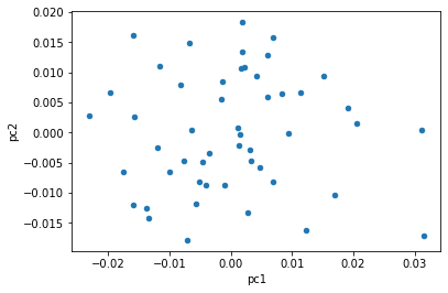
Unfortunately, this doesn’t really give us any more information about the distribution of players, it looks like it’s just randomly scattered across the grid.
My next approach was to see if the moves are separable by player. In other words, do each of our players have a distinct, significant style associated with their moves? In order to test this, I built a few multi-class classification models using scikit-learn, to see if we can actually predict which of the players in my dataset played an unseen move. It turns out that building classification models in scikit-learn is very very easy! Just look at the following code:
cross_val_score(RandomForestClassifier(), X1, y)
cross_val_score(LogisticRegression(), X1, y)
cross_val_score(KNeighborsClassifier, X1, y)
In just three lines of code, we’ve built three different classification models - Random Forests, Logistic Regression, and KNN. We've also trained each of them on the input features `X1` and classes `y`, applied k-fold cross validation on each of the models, and calculated accuracy scores for each of the models.
I ended up training 9 models, 3 models for each of the datasets X1, X2, and X3. X1 represents the move that the player made, X2 represents the move that the engine chooses, and X3 represents the difference between these two moves, a basic representation of player bias. Here are the accuracy results from the models!
Random Forest
0.031 - Player Change
0.029 - Optimal Change
0.024 - Player Bias

Logistic Regression
0.023 - Player Change
0.022 - Optimal Change
0.022 - Player Bias

KNN
0.026 - Player Change
0.026 - Optimal Change
0.020 - Player Bias
Yes, you're reading that right - those accuracy values are all under 4%! Ordinarily that would mean our classifier is extraordinarily bad, since we ideally try to get classifiers of 90% accuracy or more, and 50% means the model is no better than random. However, if you think about it, the classifier is given a new move, and asked to predict which of the 50 players the new move was made by, so a random classifier would only get 2% accuracy. 2.5-3% accuracy means that we have made some marginal improvement over random. Overall, this means that our classifier is not extraordinarily bad, but just bad.
We can compare the three models and see that random forest seems to be performing the best. It is also relatively quick to train, taking about 1-2 minutes for each model, so we'll be sticking with random forests in the future.
It also looks like player change is the most separable category of moves, not player bias as I would have expected. The first interpretation of this that comes to mind is that players don't tend to play different styles of moves. Rather, they tend to get into different types of positions which call for different styles to be played according to an optimal engine. This is supported by the fact that optimal engines are still classifiable based on the player, even though an engine should be playing the same moves for any given board state.
My next step was to add some more information to the model, in addition to the move itself, to see if the accuracy would go up. The two pieces of information I decided to add was the piece moved (king/queen/bishop/knight/rook/pawn), and the current position. To see which of these was most useful, I ended up creating 4 models - the move by itself, move+piece, move+position, and move+piece+position. I did this for the three categories of move comparisons (player move, optimal move, player bias), to get a total of 12 models. Here are the results:
Baseline Accuracy: 0.020

Move Vector Only
0.031 - Player Change
0.029 - Optimal Change
0.024 - Player Bias

Move Vector and Piece Moved
0.032 - Player Change
0.031 - Optimal Change
0.023 - Player Bias

Move Vector and Initial Position
0.038 - Player Change
0.036 - Optimal Change
0.033 - Player Bias

Move Vector, Piece Moved, and Initial Position
0.037 - Player Change
0.035 - Optimal Change
0.034 - Player Bias
While we did see an improvement with these values, one of the issues is that these values are simply too low to really understand, since all of the values have a baseline of 1/50=2%. In addition, this approach does not scale very well when we add new players. If we are operating on a dataset of a million players, we aren't going to be comparing accuracy values to the nearest 0.000001%, this isn't even a meaningful number over a dataset of a few thousand games (or fewer) per player.
The other reason this doesn't make sense is in the end, we don't really even care about comparing players to other individuals - we want to understand player styles, and how players are similar to each other. If this sounds like a clustering problem to you, we're on the same page! I decided to run all the player's mean values through the scikit-learn Kmeans algorithm. Then, instead of using the player name as the output class, we can then use the player's cluster number as the class. This way, we aren't doing a 50-class classification problem, just 2 classes. Learning the same 12 models as before, we the following results:
Baseline Accuracy: 0.500

Move Vector Only
0.612 - Player Change
0.604 - Optimal Change
0.540 - Player Bias

Move Vector and Piece Moved
0.612 - Player Change
0.630 - Optimal Change
0.642 - Player Bias

Move Vector and Initial Position
0.600 - Player Change
0.601 - Optimal Change
0.588 - Player Bias

Move Vector, Piece Moved, and Initial Position
0.602 - Player Change
0.601 - Optimal Change
0.583 - Player Bias
We can see here that the results are much higher than 3% accuracy, they are now up to about 60% accuracy because of the class reduction. I'm not quite sure if the 60% is an actual improvement, but it seems interesting so far. I have a few ideas on how to improve the model, but you'll have to wait until next time to see what I have in mind! If you want to check out the actual code, you can find it at https://github.com/saumikn/learning-chess-biases/.
See you all next week!


0 Comments