Summary
For this project, I analyzed methods to model the aleatoric and epistemic uncertainty of a neural network model for predicting the amount of time that a human player will use for a given move in a chess position.
Dataset
The dataset for these experiments comes from Lichess, an open-source chess server, and one of the most popular chess websites in the world. Lichess freely makes available all of the games which have been played on the website since January 2013, a total of about 2.07 billion games. However, none of the games before April 2017 include metadata about move times. In this study, we limit ourselves to data since April 2017, about 1.92 billion games. These data files are stored as compressed text files, and take up about 455GB of storage space.
While the raw data takes up a reasonable amount of space, extracting useful features quickly balloons the amount of storage space needed. Consider the following sample game from the data:
[Event "Rated Bullet tournament https://lichess.org/tournament/yc1WW2Ox"]
[Site "https://lichess.org/PpwPOZMq"]
[Date "2017.04.01"]
[Round "-"]
[White "Abbot"]
[Black "Costello"]
[Result "0-1"]
[UTCDate "2017.04.01"]
[UTCTime "11:32:01"]
[WhiteElo "2100"]
[BlackElo "2000"]
[WhiteRatingDiff "-4"]
[BlackRatingDiff "+1"]
[WhiteTitle "FM"]
[ECO "B30"]
[Opening "Sicilian Defense: Old Sicilian"]
[TimeControl "300+0"]
[Termination "Time forfeit"]

1. e4 { [%eval 0.17] [%clk 0:00:30] } 1... c5 { [%eval 0.19] [%clk 0:00:30] }
2. Nf3 { [%eval 0.25] [%clk 0:00:29] } 2... Nc6 { [%eval 0.33] [%clk 0:00:30] }
3. Bc4 { [%eval -0.13] [%clk 0:00:28] } 3... e6 { [%eval -0.04] [%clk 0:00:30] }
4. c3 { [%eval -0.4] [%clk 0:00:27] } 4... b5? { [%eval 1.18] [%clk 0:00:30] }
5. Bb3?! { [%eval 0.21] [%clk 0:00:26] } 5... c4 { [%eval 0.32] [%clk 0:00:29] }
6. Bc2 { [%eval 0.2] [%clk 0:00:25] } 6... a5 { [%eval 0.6] [%clk 0:00:29] }
7. d4 { [%eval 0.29] [%clk 0:00:23] } 7... cxd3 { [%eval 0.6] [%clk 0:00:27] }
8. Qxd3 { [%eval 0.12] [%clk 0:00:22] } 8... Nf6 { [%eval 0.52] [%clk 0:00:26] }
9. e5 { [%eval 0.39] [%clk 0:00:21] } 9... Nd5 { [%eval 0.45] [%clk 0:00:25] }
10. Bg5?! { [%eval -0.44] [%clk 0:00:18] } 10... Qc7 { [%eval -0.12] [%clk 0:00:23] }
11. Nbd2?? { [%eval -3.15] [%clk 0:00:14] } 11... h6 { [%eval -2.99] [%clk 0:00:23] }
12. Bh4 { [%eval -3.0] [%clk 0:00:11] } 12... Ba6? { [%eval -0.12] [%clk 0:00:23] }
13. b3?? { [%eval -4.14] [%clk 0:00:02] } 13... Nf4? { [%eval -2.73] [%clk 0:00:21] } 0-1
There are 26 different chess positions embedded in this single game example, one position for each move for both white and black. Each position is represented by a 13x64 matrix, seven additional 13x64 matrices which designate the previous seven board states, an 1858-length feature to represent legal moves in the position, and approximately nineteen relevant metadata values which are held constant through the entire game. Reshaping the data to give us a valid matrix shape for a neural network, we end up with a 123x64 floating point matrix. If we were to store the complete data for each matrix in storage, this would occupy over 760 TB of storage.
Since our data is very sparse, using an off-the-shelf data compressor such as GZIP does help, and reduces the storage requirement to only 20TB. However, this is still too large for our storage capabilities. More importantly, loading compressed files is extremely slow and immediately leads to memory shortages, since our files are far too big to load into memory.
Feature Extraction
To solve these issues, I employed a number of techniques to reduce the size of the data. First, I took advantage of the binary board representation and the np.packbits() function to compress eight boolean values into a single byte of memory. I also used np.packbits() to store the 1858-length legal moves feature into a 233-length byte array, and to compress five boolean metadata values for a board position into a single byte of memory. I also extracted the other non-binary numeric metadata from the array and saved them as corresponding arrays with either uint8 or uint16 datatypes, rather than the default \pyth{int64}. Finally, I replaced all of the prior board states associated with the current position with pointers to other board states, so we only need to store one 13x64 matrix per position, not eight 13x64 matrices.
I then saved all of these data pieces into a Hierarchical Data Format (HDF5) file. HDF5 has two main benefits - I can load chunks of compressed data into memory without overfilling the system, and I can group batches of games together to improve saving and loading time. Specifically, I'm loading files into batches of 10,000 games, or about 65,000 positions per batch.
When it's time to actually train our models, we need to correctly reconstruct our data. I set up a Keras Data Generator which correctly retrieves the prior positions and positions the metadata correctly into the 123x64 matrix.
Because the reconstruction process was operating quite slowly, I implemented my reconstruction code in Numba to speed up this process. Using Numba, I was able to speed up this processing time by over 10x.
In the end, I created a pipeline which can correctly extract features from raw data, compress these features into an HDF5 file, and efficiently load batches of features into Keras to call while fitting a model.
Baseline Model
As my baseline model for this project, I created a simple fully-connected neural network, which took in an input vector of length 19. This vector represents eight dimensions for position metadata, nine dimensions for game metadata, and two dimensions for current time metadata.
Specifically, my model has three hidden layers with an output size of 32, each followed by the ReLu activation function. The final layer is another dense layer with an output size of 1, for my final point estimate of the move time. I used the RMSprop optimizer and an initial learning rate of 0.001.
Originally, my plan was to train a convolutional neural network, but this fell through when I was not able to successfully implement a Bayesian convolutional neural network (described in the next section).
Uncertainty
For this project, I investigated two sources of uncertainty of a standard neural network model, trained to predict the amount of time that a human player will use for a given move in a chess position.
Aleatoric Uncertainty
The first uncertainty I investigated was aleatoric uncertainty. In plain English, this is the uncertainty caused by randomness inherent to the domain. Because this uncertainty is inherent to the domain, it can never be reduced, no matter how much data we have.
In the domain of move time predictions, an example of aleatoric uncertainty would be that, for a given position, different players will likely use different amounts of time for the same move. Even if we are given an infinite-sized dataset, and we standardize every possible variable that we have in our dataset - game metadata, position data, and position metadata - we will still never perfectly predict the amount of movetime taken.
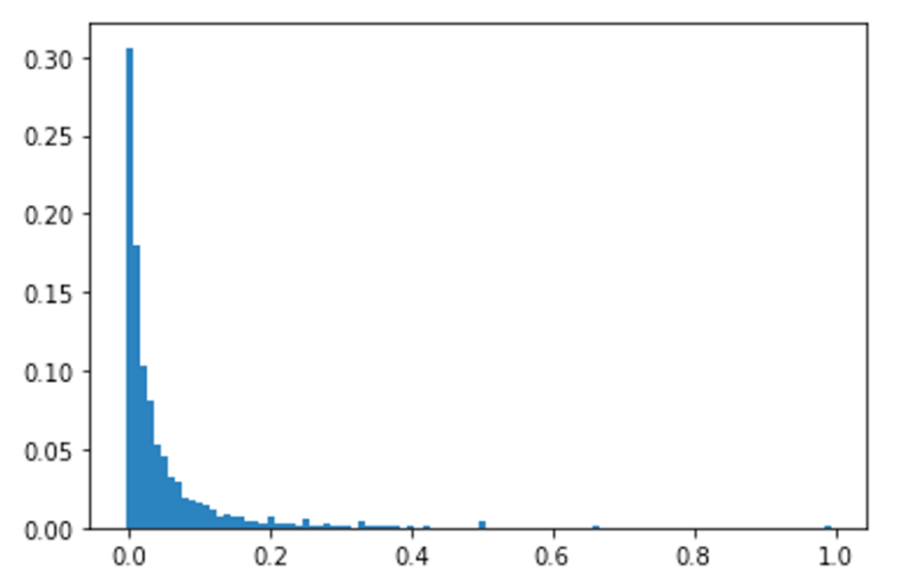
To deal with this issue, we can try to predict a distribution as the output of our model, instead of a single point estimate. The below graph shows the distribution of all moves in our dataset.

While a number of distributions could potentially model our dataset, I decided to use the beta distribution for the key reason that it is constrained between 0 and 1, just like our data. Other distributions such as the log-normal distribution or the exponential distribution could work well too, but I thought that their tails would bias the model too much.
To train our model with a beta distribution, we can no longer use Mean Absolute Error (MAE), since MAE only works with point estimates. Instead, I trained my beta distribution predictor with the Conditional Ranked Probability Score (CRPS) loss function. The main benefit of CRPS is it can simply be treated as a probabilistic extension of MAE, so we can easily compare losses between our point estimate and distribution estimate.
Initially, I used the crps_quadrature method in Python's \pyth{properscoring} module to calculate the CRPS. However, this numerical integration approximation was proving to be quite slow. Instead, I found a closed-form solution for the CRPS of a Beta distribution, provided in the paper Taillardat et al (2016). Below is my implementation of the formula in Python.
from scipy.special import gamma as G
from scipy.stats import beta
def crps_beta(y, pred):
    a, b = pred
    cdf0 = beta(a,b).cdf
    cdf1 = beta(a+1,b).cdf

    return a/(a+b) * (1-2*cdf1(y)) \
        - y * (1-2*cdf0(y)) \
        - 1/(a+b) * G(a+b)*G(a+0.5)*G(b+0.5)/(np.sqrt(np.pi)*G(a+b+0.5)*G(a)*G(b))
Epistemic Uncertainty
The second type of uncertainty I investigated was epistemic uncertainty. This represents the uncertainty as a result of low data. To model this uncertainty, I used a Bayesian neural network.
My neural network (described above) retained the same structure as above, with three hidden dense layers with output size 32, and the same training hyperparameters. The only difference is that each dense layer represented a distribution instead of a single value. Each parameter was given a prior normal distribution, with mean 0 and standard deviation 1.
Results
My first result comes from the investigation on aleatoric uncertainty. In the end, I found that my point estimate network had a final loss function of 3.59%, while the beta distribution estimate had a final loss function of 5.19%.
This was quite surprising, as we would intuitively expect that the distribution network encodes more information about the prediction than a simple point estimate does. After thinking about this for some time, my explanation for this is that a beta distribution is simply a bad model for the data. With hindsight, modeling my data with an exponential distribution would have been a much better choice. While it's true that the exponential distribution extends past 1, this tail should take up a very small amount of the data overall, and the fact that the exponential distribution looks to fit the majority of the data means that it should pose better predictive qualities.
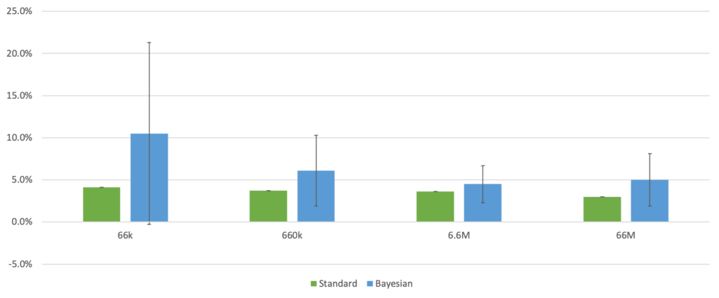
My second result comes from the investigation on epistemic uncertainty. The below graph shows my results.

I trained four pairs of models, on four different orders of magnitude data size. For each data selection, the standard model drastically outperformed the Bayesian model. As we get more data, the Bayesian model does perform relatively better, and the uncertainty of the model diminishes tends to diminish, though it unexpectedly rises again with n = 66 million.
Conclusion
Overall, we found negative results for our investigations on both aleatoric and epistemic uncertainty. For the former, we found that modeling our prediction as a beta distribution produced worse results than a point estimate. For the latter, we found that structuring our neural network as a Bayesian NN produced worse results than a standard neural network.
The obvious next step for this project is to inspect our results from the project in more depth. On the aleatoric side, I would like to try modeling the data using other distribution types, most notably the exponential distribution. On the epistemic side, I would like to explore using different priors for our parameters, rather than just a normal distribution.
More long-term, I would like to explore using a more complicated model like a CNN, so I can include the board information as well. After that, the next steps are to retrain models on personalized datasets, so I can start to develop better teaching tools.


0 Comments